Prior to making any statistical interference, the distribution of the metal and TSS data is required to be assessed if outlier concentrations are present due to variability in the measurement or experimental error. This pre-processing procedure is referred to as:
Data Normalization
The goal of normalization is to change the values of numeric columns in the dataset to a common scale, without distorting differences in the ranges of values. The normalization approach to a data set is required to accurately report trends in the data when the overall distribution is not Gaussian (a bell curve). In order to confirm whether data needs normalization for the distribution of metal concentrations, the Shapiro-Wilk test for normality was performed on the data set.
Shapiro-Wilk test
The Shapiro-Wilk test is a routine statistical assessment that quantifies the similarity between the observed and normal distributions as a single number which:
superimposes a normal curve over the observed distribution (Figure 1).
It then computes which percentage of our sample overlaps with it:
a similarity percentage.
Finally, the Shapiro-Wilk test computes the probability of finding this observed -or a smaller- similarity percentage. It does so under the assumption that the metal concentration distribution is exactly normal:
the null hypothesis.
The null hypothesis for the Shapiro-Wilk test is that a variable is normally distributed in some population. The null hypothesis is rejected if p < 0.05. If the null hypothesis is rejected, we conclude that our metal concentration is NOT normally distributed.
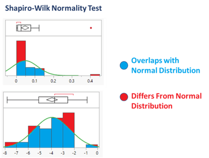 Figure 1 – Shapiro-Wilk Normality Test visualization of similarity percentage for the distribution of Arsenic (As) before (top) and after (top) log normalization. The illustration demonstrates that the log normalization of metal data increases the similarity percentage, while producing a Gaussian distribution.
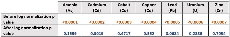 Table 1 – Shapiro-Wilk test results for metals before and after log normalization.
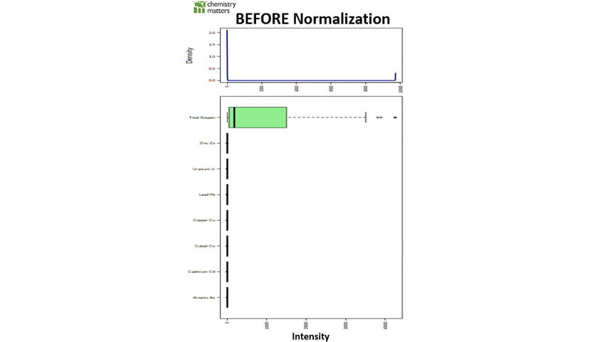
Since the p values are less than 0.05, the Shapiro-Wilk Test confirms that all the metal concentrations are not normally distributed (Table 1). As illustrated in the distribution of the pipeline data for metals with TSS (Figure 2; left), the distribution is highly skewed as a result of the relative increase in TSS concentration. When further analysis such as multivariate linear regression is conducted, the attributed concentration of TSS will intrinsically influence the results more due to its larger distribution. If data does not exhibit normal distribution, parametric statistics or regression analysis cannot be used to examine the relationship between metals and TSS.
As the study parameters are to assess the relationship between metals and TSS, the data needs to be normalized so that the null hypothesis can be accepted. This is accomplished by Logarithmic (Log) transformation of the data, which results in a common scale without distorting differences in the ranges of values. After this transformation, the data exhibits an increased similarity percentage (Figure 1), Shapiro-Wilk Test results confirming the null hypothesis that the data is distributed normally (Table 1) and distributions become scaled evenly (Figure 2).
Case Study: How Results Differ Before & After Normalization
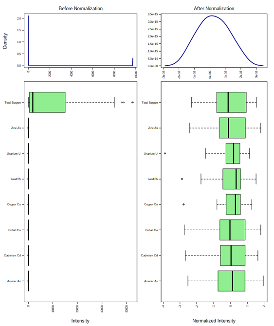 Figure 2 – Box plots and kernel density plots before (left) and after normalization (right) illustrating the range distribution in metal and TSS concentrations.


